Future of the Network Documentary

Part 1 - M2M and the Internet of Things: Brace for Impact

Part 2 - Broadband Capacity: Are We Ready?

Part 3 - Uncovering Software-Defined Networking

Part 4 - The Cloud: Building in Mid-Air

Part 5 - The Value Chain: Building Value in the Chain

Evaluating Network Gear Performance

 

Choosing the right equipment for your network is hard. Even ignoring the ever-growing roster of features one must account for when evaluating candidate hardware, it's important not to overlook performance limitations. Below are some of the most crucial characteristics to consider when doing your research.

Throughput

Throughput is the rate at which a device can convert input to output. This is different from bandwidth, which is the rate at which data travels across a medium. An Ethernet switch, for example, might have 48 ports running at an individual bandwidth of 1 Gbps each but be able to switch only a total of 12 Gbps among the ports at any given time. This is said to be the switch's maximum throughput.

 

Throughput is measured in two units: bits per second (bps) and packets per second (pps). Most people are most familiar with bits per second. This is the amount of data which flows through a particular point within a duration of one second, typically expressed as megabits (Mbps) or gigabits (Gbps) per second. Capitalization is important here. A lowercase 'b' indicates bits, whereas an uppercase 'B' indicates bytes. Speed is always measured in bits per second, with a lowercase 'b' (Kbps or Mbps).

 

Packets per second, similarly expressed most often as Kpps or Mpps, is another way of evaluating throughput. It conveys the number of packets or frames which can be processed in one second. This approach to measuring throughput is used to expose limitations of the processing power of devices, as shorter packets demand more frequent forwarding decisions. For example, a router might claim a throughput of 30 Mbps per second using full-size packets. However, it might also be limited to processing 40 Kpps. If each packet received was the minimum size of 64 bytes (512 bits), the router would be limited to just 20.48 Mbps (512 * 40,000) of throughput.

 

Cisco maintains often cited baseline performance measurements for its most popular routers and switches. If you work out the math, you can see that the Mbps numbers listed in the router performance document were derived using minimum-length (64 byte) packets. These numbers thus present a worst case scenario. Packets on a production network typically vary widely in size, and larger packets will yield higher bits-per-second rates.

 

Keep in mind that these benchmarks were taken with no features other than IP routing enabled. Adding additional features and services such as access control lists or network address translation may reduce throughput. Unfortunately, it's impractical for a vendor to list throughput rates with and without myriad features enabled, so you'll have to do some testing yourself.

Oversubscription

Ethernet switches are often built with oversubscribed backplanes. Oversubscription refers to a point of congestion within a system where the potential rate of input is greater than the potential rate of output. For example, a switch with 48 1 Gbps ports might have a backplane throughput limitation of only 16 Gbps. This means that only 16 ports can transmit at wire rate (the physical maximum throughput) at any point in time. This isn't usually a problem at the network edge, where few users or servers ever need to transmit at these speeds for a prolonged time. However, oversubscription imposes much more critical considerations in the data center or network core.

 

As an example, let's look at the 16-port 10 Gbps Ethernet module WS-X6816-10G-2T for the Cisco Catalyst 6500 switch. Although the module provides an aggregate of 160 Gbps of potential throughput, its connection to the chassis backplane is only 40 Gbps. The module is oversubscribed at a ratio of 4:1. This module should only be used in situations where the aggregate throughput demand from all interfaces is not expected to exceed 40 Gbps.

IP Route Capacity

The maximum number of routes a router can hold in its routing table is limited by the amount of available content-addressable memory (CAM). Although a low-end router may be able to run BGP and exchange routes with BGP peers, it likely won't have sufficient memory to accept the full IPv4 Internet routing table, which comprises over 400 thousand routes. (Of course, low-end routers should never be implemented in a position where they would need to receive the full routing table.) Virtual routing contexts, in which a router stores multiple copies of a route in separate forwarding tables, increase routing table size exponentially, further elevating the importance of properly sizing routers for the role they play.

Maximum Concurrent Sessions

Firewalls and intrusion prevention systems perform stateful inspection of traffic transiting from one trust zone to another. These devices must be able to keep up with the demand for throughput not only in terms of bits per second and packets per second but also in the number of concurrent stateful sessions. A single web request might trigger the initiation of one or two dozen TCP connections to various content servers from an internal host. The firewall or IPS must be able to track the state of and inspect potentially thousands of sessions at any point in time. If the device's maximum capacity is reached, attempts to open new sessions may be rejected until a number of current sessions are closed or expire. Such devices are likewise limited in how fast they can create new sessions.

 

The Science of Network Troubleshooting

Courtesy - Jemery Stretch

 

Troubleshooting is not an art. Along with many other IT methodologies, it is often referred to as an art, but it's not. It's a science, if ever there was one. Granted, someone with great skill in troubleshooting can make it seem like a natural talent, the same way a professional ball player makes hitting a home run look easy, when in fact it is a learned skill. Another common misconception holds troubleshooting as a skill derived entirely from experience with the involved technologies. While experience is certainly beneficial, the ability to troubleshoot effectively arises primarily from the embrace of a systematic process, a science.

 

It's said that troubleshooting can't be taught, but I disagree. More accurately, I would argue that troubleshooting can't be taught easily, or to great detail. This is because traditional education encompasses how a technology functions; troubleshooting encompasses all the ways in which it can cease to function. Given that it's virtually impossible to identify and memorize all the potential points of failure a system or network might hold, engineers must instead learn a process for identifying and resolving malfunctions as they occur. To borrow a cliché analogy, teach a man to identify why a fish is broken, rather than expecting him to memorize all the ways a fish might break.

Troubleshooting as a Process

Essentially, troubleshooting is the correlation between cause and effect. Your proxy server experiences a hard disk failure, and you can no longer access web pages. A backhoe digs up a fiber, and you can't call a branch office. Cause, and effect. Moving forward, the correlation is obvious; the difficulty lies in transitioning from effect to cause, and this is troubleshooting at its core.

 

Consider walking into a dark room. The light is off, but you don't know why. This is the observed effect for which we need to identify a cause. Instinctively, you'll reach for the light switch. If the light switch is on, you'll search for another cause. Maybe the power is out. Maybe the breaker has been tripped. Maybe someone stole all the light bulbs (it happens). Without much thought, you investigate each of these possible causes in order of convenience or likelihood. Subconsciously, you're applying a process to resolve the problem.

 

Even though our light bulb analogy is admittedly simplistic, it serves to illustrate the fundamentals of troubleshooting. The same concepts are scalable to exponentially more complex scenarios. From a high-level view, the troubleshooting process can be reduced to a few core steps:

• Identify the effect(s)
• Eliminate suspect causes
• Devise a solution
• Test and repeat
• Mitigate

Step 1: Identify the Effect(s)

If you've been a network engineer for more than a few hours, you've been told at least once that the Internet is down. Yes, the global information infrastructure some forty years in the making has fallen to its knees and is in a state of complete chaos. All this is, of course, confirmed by Mary in accounting. Last time it was discovered her Ethernet cable had come unplugged, but this time she's certain it's a global catastrophe.

 

Correctly identifying the effects of an outage or change is the most critical step in troubleshooting. A poor judgment at this first step will likely start you down the wrong path, wasting time and resources. Identifying an effect is not to be confused with deducing a probable cause; in this step we are focused solely on listing the ways in which network operation has deviated from the norm.

 

Identifying effects is best done without assumption or emotion. While your mind will naturally leap to possible causes at the first report of an outage, you must force yourself to adopt an objective stance and investigate the noted symptoms without bias. In the case of Mary's doomsday forecast, you would likely want to confirm the condition yourself before alerting the authorities.

Some key points to consider:

What was working and has stopped?

An important consideration is whether an absent service was ever present to begin with. A user may report an inability to reach FTP sites as an outage, not realizing FTP connections have always been blocked by the firewall as a matter of policy.

What wasn't working and has started?

This is can be a much less obvious change, but no less important. One example would be the easing of restrictions on traffic types or bandwidth, perhaps due to routing through an alternate path, or the deletion of an access control mechanism.

What has continued to work?

Has all network access been severed, or merely certain types of traffic? Or only certain destinations? Has a contingency system assumed control from a failed production system?

When was the change observed?

This critical point is very often neglected. Timing is imperative for correlation with other events, as we'll soon see. Also remember that we are often limited to noting the time a change was observed, rather than when it occurred. For example, an outage observed Monday morning could have easily occurred at any time during the preceding weekend.

Who is affected? Who isn't?

Is the change limited to a certain group of users or devices? Is it constrained to a geographical or logical area? Is any person or service immune?

Is the condition intermittent?

Does the condition disappear and reappear? Does this happen at predictable intervals, or does it appear to be random?

Has this happened before?

Is this a recurring problem? How long ago did it happen last? What was the resolution? (You do keep logs of this sort of thing, right?)

Correlation with planned maintenance and configuration changes

Was something else being changed at this time? Was a device added, removed, or replaced? Did the outage occur during a scheduled maintenance window, either locally or at another site or provider?

Step 2: Eliminate Suspect Causes

Once we have a reliable account of the effect or effects, we can attempt to deduce probable causes. I say probable because deducing all possible causes is impractical, if not impossible. One possible cause is a power failure. Another possible cause is spontaneous combustion. Only one of these possible causes is probable.

 

There is a popular mantra of "always start with layer one," suggesting that the physical connectivity of a network should be verified before working on the higher layers. I disagree, as this is misleading and often impractical. You're not going to drive out to a remote site to verify everything is plugged in if a simple ping verifies end-to-end connectivity. Similarly, it's unlikely that any cables were disturbed if you can verify with relative certainty no one has gone near the suspect devices. Perhaps this is an oversimplified argument, but verifying physical connectivity is often needlessly time consuming and superseded by alternative methods.

 

Instead, I suggest narrowing causes in order of combined probability and convenience. For example, there might be nothing to indicate DNS is returning an invalid response, but performing a manual name resolution takes roughly two seconds, so this is easily justified. Conversely, comparing a current device configuration to its week-old backup and accounting for any differences may take a considerable amount of time, but this presents a high probability of exposing a cause, so it too is justified.

 

The order in which you decide to eliminate suspect causes is ultimately dependent on your experience, your familiarity with the infrastructure, and your allowance for time. Regardless of priority, each suspect cause should undergo the same process of elimination:

Define a working condition

You can't test for a condition unless you know what condition to expect. Before performing a test, you should have in mind what outcome should be produced in the absence of an outage. For example, performing a traceroute to a distant node is meaningless if you can't compare it against a traceroute to the same destination under normal conditions.

Define a test for that condition

Ensure that the test you perform is in fact evaluating the suspect cause. For instance, pinging an E-mail server doesn't explicitly guarantee that mail services are available, only the server itself (technically, only that server's address). To verify the presence of mail services, a connection to the relevant daemon(s) must be established.

Apply the test and record the result

Once you've applied the test, record its success or failure in your notes. Even if you've eliminated the cause under suspicion, you have a reference to remind you of this and avoid wasting time repeating the same test again unnecessarily.

It is common to uncover multiple failures in the course of troubleshooting. When this happens, it is important to recognize any dependencies. For example, if you discover that E-mail, web access, and a trunk link are all down, the E-mail and web failures can likely be ignored if they depend on the trunk link to function. However, always remember to verify these supposed secondary outages after the primary outage has been resolved.

Step 3: Devise a Solution

Once we have identified a point of failure, we want to continue our systematic approach. Just as with testing for failures, we can apply a simple methodology to testing for solutions. In fact, the process very closely mirrors the steps performed to eliminate suspect causes.

Define the failure

At this point you should have a comfortable idea of the failure. Form a detailed description so you have something to test against after applying a solution. For example, you would want to refine "The Internet is down" to "Users in building 10 cannot access the Internet because their subnet was removed from the outbound ACL on the firewall."

Define the proposed solution

Describe exactly what changes are to be made, and exactly what the expected outcome is. Blanket solutions such as arbitrarily rebooting a device or rebuilding a configuration from scratch might fix the problem, but they prevent any further diagnosis and consequently impede mitigation.

Apply the solution and record the result

Once we have a defined failure and a proposed solution, it's time to pit the two against each other. Be observant in applying the solution, and record its result. Does the outcome match what you expected? Has the failure been resolved?

In addition to our defined process, some guidelines are well worth mentioning.

Maintain focus

Far too often I encounter a technician who, upon becoming frustrated with a failure or failures, opts to recklessly reboot, reconfigure, or replace a device instead of troubleshooting systematically. This is the high-tech equivalent of pounding something with a hammer until it works. Focus on one failure at a time, and one solution at a time per failure.

Watch out for hazardous changes

When developing a solution, remember to evaluate what effect it might have on systems unrelated to those being troubleshot. It's a horrible feeling to realize you've fixed one problem at the expense of causing a much larger one. The best course of action when this happens is typically to immediately reverse the change which was made. Note that this is only possible with a systematic approach.

Step 4: Test and Repeat

Upon implementing a solution and observing a positive effect, we can begin to retrace our steps back toward the original symptoms. If any conditions were overlooked because they were decided to be dependent on the recently resolved failure, test for them again. Refer to your notes from the initial report and verify that each symptom has been resolved. Ensure that the same tests which were used to identify a failure are used to confirm functionality.

 

If you notice that a failure or failures remain, pick up where you left off in the testing cycle, annotate it, and press forward.

Step 5: Mitigate

The troubleshooting process does not end when the problem has been resolved and everyone is happy. All of your hard work up until this point amounts to very little if the same problem occurs again tomorrow. In IT, problems are commonly fixed without ever being resolved. Band-aids and hasty installations are not acceptable substitutes for implementing a permanent and reliable solution. So to speak, many people will go on mopping the floor day after day without ever plugging the leak.

 

A permanent solution may be as complex as redesigning the routed backbone, or as simple as moving a power strip somewhere it won't be tripped on anymore. A permanent solution also doesn't have to be 100% effective, but it should be as effective as is practical. At the absolute minimum, ensure that you record the observed failure and the applied solution, so that if it the condition does recur you have an accurate and dated reference.

A Final Word

Everyone has his or her own preference in troubleshooting, and by no means do I consider this paper conclusive. However, if there's only one concept you take away, make it this: above all else, remain calm. You're no good to anyone in a panic. One's ability to manage stress and maintain a professional demeanor even in the face of utter chaos is what makes a good engineer great.

 

Most network outages, despite what we're led to believe by senior management, are not the end of the world. There are instances where downtime can lead to loss of life; fortunately, this isn't the case with the vast majority of networks. Money may be lost, time may be wasted, and feelings may be hurt, but when the problem is finally resolved, odds are you've learned something valuable.

 

Wireless 101 - Part 2

Antenna

An antenna is a device to transmit and/or receive electromagnetic waves. Electromagnetic waves are often referred to as radio waves. Most antennas are resonant devices, which operate efficiently over a relatively narrow frequency band. An antenna must be tuned (matched) to the same frequency band as the radio system to which it is connected otherwise reception and/or transmission will be impaired.

Types of antenna

There are 3 types of antennas used with mobile wireless, omnidirectional, dish and panel antennas.
+ Omnidirectional radiate equally in all directions
+ Dishes are very directional
+ Panels are not as directional as Dishes.



Decibels

Decibels (dB) are the accepted method of describing a gain or loss relationship in a communication system. If a level is stated in decibels, then it is comparing a current signal level to a previous level or preset standard level. The beauty of dB is they may be added and subtracted. A decibel relationship (for power) is calculated using the following formula:

“A” might be the power applied to the connector on an antenna, the input terminal of an amplifier or one end of a transmission line. “B” might be the power arriving at the opposite end of the transmission line, the amplifier output or the peak power in the main lobe of radiated energy from an antenna. If “A” is larger than “B”, the result will be a positive number or gain. If “A” is smaller than “B”, the result will be a negative number or loss.

You will notice that the “B” is capitalized in dB. This is because it refers to the last name of Alexander Graham Bell.

Note:

+ dBi is a measure of the increase in signal (gain) by your antenna compared to the hypothetical isotropic antenna (which uniformly distributes energy in all directions) -> It is a ratio. The greater the dBi value, the higher the gain and the more acute the angle of coverage.

+ dBm is a measure of signal power. It is the the power ratio in decibel (dB) of the measured power referenced to one milliwatt (mW). The “m” stands for “milliwatt”.

Example:

At 1700 MHz, 1/4 of the power applied to one end of a coax cable arrives at the other end. What is the cable loss in dB?

Solution:

=> Loss = 10 * (- 0.602) = – 6.02 dB

From the formula above we can calculate at 3 dB the power is reduced by half. Loss = 10 * log (1/2) = -3 dB; this is an important number to remember.

Beamwidth

The angle, in degrees, between the two half-power points (-3 dB) of an antenna beam, where more than 90% of the energy is radiated.

OFDM

OFDM was proposed in the late 1960s, and in 1970, US patent was issued. OFDM encodes a single transmission into
multiple sub-carriers. All the slow subchannel are then multiplexed into one fast combined channel.

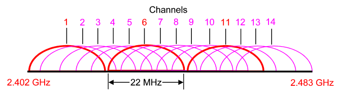
The trouble with traditional FDM is that the guard bands waste bandwidth and thus reduce capacity. OFDM selects channels that overlap but do not interfere with each other.



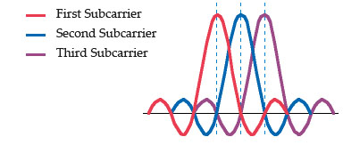
OFDM works because the frequencies of the subcarriers are selected so that at each subcarrier frequency, all other subcarriers do not contribute to overall waveform.

In this example, three subcarriers are overlapped but do not interfere with each other. Notice that only the peaks of each subcarrier carry data. At the peak of each of the subcarriers, the other two subcarriers have zero amplitude.

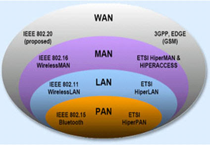
Types of network in CCNA Wireless

+ A LAN (local area network) is a data communications network that typically connects personal computers within a very limited geographical (usually within a single building). LANs use a variety of wired and wireless technologies, standards and protocols. School computer labs and home networks are examples of LANs.

+ A PAN (personal area network) is a term used to refer to the interconnection of personal digital devices within a range of about 30 feet (10 meters) and without the use of wires or cables. For example, a PAN could be used to wirelessly transmit data from a notebook computer to a PDA or portable printer.

+ A MAN (metropolitan area network) is a public high-speed network capable of voice and data transmission within a range of about 50 miles (80 km). Examples of MANs that provide data transport services include local ISPs, cable television companies, and local telephone companies.

+ A WAN (wide area network) covers a large geographical area and typically consists of several smaller networks, which might use different computer platforms and network technologies. The Internet is the world’s largest WAN. Networks for nationwide banks and superstore chains can be classified as WANs.

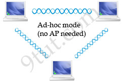
Bluetooth

Bluetooth wireless technology is a short-range communications technology intended to replace the cables connecting portable and/or fixed devices while maintaining high levels of security. Connections between Bluetooth devices allow these devices to communicate wirelessly through short-range, ad hoc networks. Bluetooth operates in the 2.4 GHz unlicensed ISM band.

Note:

Industrial, scientific and medical (ISM) band is a part of the radio spectrum that can be used by anybody without a license in most countries. In the U.S, the 902-928 MHz, 2.4 GHz and 5.7-5.8 GHz bands were initially used for machines that emitted radio frequencies, such as RF welders, industrial heaters and microwave ovens, but not for radio communications. In 1985, the FCC Rules opened up the ISM bands for wireless LANs and mobile communications. Nowadays, numerous applications use this band, including cordless phones, wireless garage door openers, wireless microphones, vehicle tracking, amateur radio…

WiMAX

Worldwide Interoperability for Microwave Access (WiMax) is defined by the WiMax forum and standardized by the IEEE 802.16 suite. The most current standard is 802.16e.

Operates in two separate frequency bands, 2-11 GHz and 10-66 GHz
At the higher frequencies, line of sight (LOS) is required – point-to-point links only
In the lower region, the signals propagate without the requirement for line of sight (NLOS) to customers

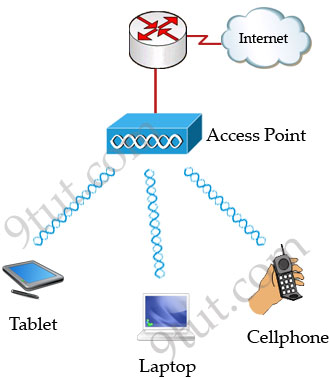
Basic Service Set (BSS)

A group of stations that share an access point are said to be part of one BSS.

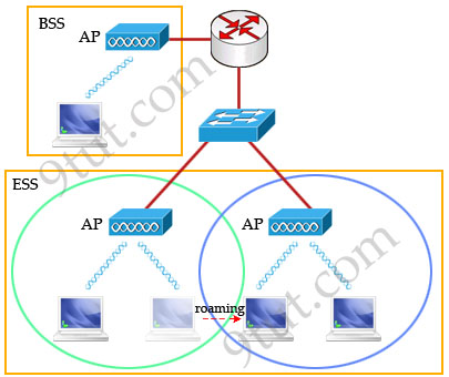
Extended Service Set (ESS)

Some WLANs are large enough to require multiple access points. A group of access points connected to the same WLAN are known as an ESS. Within an ESS, a client can associate with any one of many access points that use the same Extended service set identifier (ESSID). That allows users to roam about an office without losing wireless connection.

IEEE 802.11 standard

A family of standards that defines the physical layers (PHY) and the Media Access Control (MAC) layer.

* IEEE 802.11a: 54 Mbps in the 5.7 GHz ISM band
* IEEE 802.11b: 11 Mbps in the 2.4 GHz ISM band
* IEEE 802.11g: 54 Mbps in the 2.4 GHz ISM band
* IEEE 802.11i: security. The IEEE initiated the 802.11i project to overcome the problem of WEP (which has many flaws and it could be exploited easily)
* IEEE 802.11e: QoS
* IEEE 802.11f: Inter Access Point Protocol (IAPP)

More information about 802.11i:

The new security standard, 802.11i, which was ratified in June 2004, fixes all WEP weaknesses. It is divided into three main categories:

1. Temporary Key Integrity Protocol (TKIP) is a short-term solution that fixes all WEP weaknesses. TKIP can be used with old 802.11 equipment (after a driver/firmware upgrade) and provides integrity and confidentiality.
2. Counter Mode with CBC-MAC Protocol (CCMP) [RFC2610] is a new protocol, designed from ground up. It uses AES as its cryptographic algorithm, and, since this is more CPU intensive than RC4 (used in WEP and TKIP), new 802.11 hardware may be required. Some drivers can implement CCMP in software. CCMP provides integrity and confidentiality.
3. 802.1X Port-Based Network Access Control: Either when using TKIP or CCMP, 802.1X is used for authentication.

Wireless Access Points

There are two categories of Wireless Access Points (WAPs):
* Autonomous WAPs
* Lightweight WAPs (LWAPs)

Autonomous WAPs operate independently, and each contains its own configuration file and security policy. Autonomous WAPs suffer from scalability issues in enterprise environments, as a large number of independent WAPs can quickly become difficult to manage.

Lightweight WAPs (LWAPs) are centrally controlled using one or more Wireless LAN Controllers (WLCs), providing a more scalable solution than Autonomous WAPs.

Encryption

Encryption is the process of changing data into a form that can be read only by the intended receiver. To decipher the message, the receiver of the encrypted data must have the proper decryption key (password).

TKIP

TKIP stands for Temporal Key Integrity Protocol. It is basically a patch for the weakness found in WEP. The problem with the original WEP is that an attacker could recover your key after observing a relatively small amount of your traffic. TKIP addresses that problem by automatically negotiating a new key every few minutes — effectively never giving an attacker enough data to break a key. Both WEP and WPA-TKIP use the RC4 stream cipher.

TKIP Session Key

* Different for every pair
* Different for every station
* Generated for each session
* Derived from a “seed” called the passphrase

AES

AES stands for Advanced Encryption Standard and is a totally separate cipher system. It is a 128-bit, 192-bit, or 256-bit block cipher and is considered the gold standard of encryption systems today. AES takes more computing power to run so small devices like Nintendo DS don’t have it, but is the most secure option you can pick for your wireless network.

EAP

Extensible Authentication Protocol (EAP) [RFC 3748] is just the transport protocol optimized for authentication, not the authentication method itself:

” EAP is an authentication framework which supports multiple authentication methods. EAP typically runs directly over data link layers such as Point-to-Point Protocol (PPP) or IEEE 802, without requiring IP. EAP provides its own support for duplicate elimination and retransmission, but is reliant on lower layer ordering guarantees. Fragmentation is not supported within EAP itself; however, individual EAP methods may support this.” — RFC 3748, page 3

Some of the most-used EAP authentication mechanism are listed below:

* EAP-MD5: MD5-Challenge requires username/password, and is equivalent to the PPP CHAP protocol [RFC1994]. This method does not provide dictionary attack resistance, mutual authentication, or key derivation, and has therefore little use in a wireless authentication enviroment.
* Lightweight EAP (LEAP): A username/password combination is sent to a Authentication Server (RADIUS) for authentication. Leap is a proprietary protocol developed by Cisco, and is not considered secure. Cisco is phasing out LEAP in favor of PEAP.
* EAP-TLS: Creates a TLS session within EAP, between the Supplicant and the Authentication Server. Both the server and the client(s) need a valid (x509) certificate, and therefore a PKI. This method provides authentication both ways.
* EAP-TTLS: Sets up a encrypted TLS-tunnel for safe transport of authentication data. Within the TLS tunnel, (any) other authentication methods may be used. Developed by Funk Software and Meetinghouse, and is currently an IETF draft.
*EAP-FAST: Provides a way to ensure the same level of security as EAP-TLS, but without the need to manage certificates on the client or server side. To achieve this, the same AAA server on which the authentication will occur generates the client credential, called the Protected Access Credential (PAC).
* Protected EAP (PEAP): Uses, as EAP-TTLS, an encrypted TLS-tunnel. Supplicant certificates for both EAP-TTLS and EAP-PEAP are optional, but server (AS) certificates are required. Developed by Microsoft, Cisco, and RSA Security, and is currently an IETF draft.
* EAP-MSCHAPv2: Requires username/password, and is basically an EAP encapsulation of MS-CHAP-v2 [RFC2759]. Usually used inside of a PEAP-encrypted tunnel. Developed by Microsoft, and is currently an IETF draft.

RADIUS

Remote Authentication Dial-In User Service (RADIUS) is defined in [RFC2865] (with friends), and was primarily used by ISPs who authenticated username and password before the user got authorized to use the ISP’s network.

802.1X does not specify what kind of back-end authentication server must be present, but RADIUS is the “de-facto” back-end authentication server used in 802.1X.

Roaming

Roaming is the movement of a client from one AP to another while still transmitting. Roaming can be done across different mobility groups, but must remain inside the same mobility domain. There are 2 types of roaming:

A client roaming from AP1 to AP2. These two APs are in the same mobility group and mobility domain

Roaming in the same Mobility Group

A client roaming from AP1 to AP2. These two APs are in different mobility groups but in the same mobility domain

 

Wireless 101 - Part 1

In this article we will discuss about Wireless technologies mentioned in CCNA.

Wireless LAN (WLAN) is very popular nowadays. Maybe you have ever used some wireless applications on your laptop or cellphone. Wireless LANs enable users to communicate without the need of cable. Below is an example of a simple WLAN:

Each WLAN network needs a wireless Access Point (AP) to transmit and receive data from users. Unlike a wired network which operates at full-duplex (send and receive at the same time), a wireless network operates at half-duplex so sometimes an AP is referred as a Wireless Hub.





The major difference between wired LAN and WLAN is WLAN transmits data by radiating energy waves, called radio waves, instead of transmitting electrical signals over a cable.

Also, WLAN uses CSMA/CA (Carrier Sense Multiple Access with Collision Avoidance) instead of CSMA/CD for media access. WLAN can’t use CSMA/CD as a sending device can’t transmit and receive data at the same time. CSMA/CA operates as follows:

+ Listen to ensure the media is free. If it is free, set a random time before sending data
+ When the random time has passed, listen again. If the media is free, send the data. If not, set another random time again
+ Wait for an acknowledgment that data has been sent successfully
+ If no acknowledgment is received, resend the data

IEEE 802.11 standards:

Nowadays there are three organizations influencing WLAN standards. They are:

+ ITU-R: is responsible for allocation of the RF bands
+ IEEE: specifies how RF is modulated to transfer data
+ Wi-Fi Alliance: improves the interoperability of wireless products among vendors

But the most popular type of wireless LAN today is based on the IEEE 802.11 standard, which is known informally as Wi-Fi.

* 802.11a: operates in the 5.7 GHz ISM band. Maximum transmission speed is 54Mbps and approximate wireless range is 25-75 feet indoors.
* 802.11b: operates in the 2.4 GHz ISM band. Maximum transmission speed is 11Mbps and approximate wireless range is 100-200 feet indoors.
* 802/11g: operates in the 2.4 GHz ISM band. Maximum transmission speed is 54Mbps and approximate wireless range is 100-200 feet indoors.

ISM Band: The ISM (Industrial, Scientific and Medical) band, which is controlled by the FCC in the US, generally requires licensing for various spectrum use. To accommodate wireless LAN’s, the FCC has set aside bandwidth for unlicensed use including the 2.4Ghz spectrum where many WLAN products operate.

Wi-Fi: stands for Wireless Fidelity and is used to define any of the IEEE 802.11 wireless standards. The term Wi-Fi was created by the Wireless Ethernet Compatibility Alliance (WECA). Products certified as Wi-Fi compliant are interoperable with each other even if they are made by different manufacturers.



Access points can support several or all of the three most popular IEEE WLAN standards including 802.11a, 802.11b and 802.11g.

WLAN Modes:

WLAN has two basic modes of operation:

* Ad-hoc mode: In this mode devices send data directly to each other without an AP.

* Infrastructure mode: Connect to a wired LAN, supports two modes (service sets):

+ Basic Service Set (BSS): uses only a single AP to create a WLAN
+ Extended Service Set (ESS): uses more than one AP to create a WLAN, allows roaming in a larger area than a single AP. Usually there is an overlapped area between two APs to support roaming. The overlapped area should be more than 10% (from 10% to 15%) to allow users moving between two APs without losing their connections (called roaming). The two adjacent APs should use non-overlapping channels to avoid interference. The most popular non-overlapping channels are channels 1, 6 and 11 (will be explained later).

Roaming: The ability to use a wireless device and be able to move from one access point’s range to another without losing the connection.

When configuring ESS, each of the APs should be configured with the same Service Set Identifier (SSID) to support roaming function. SSID is the unique name shared among all devices on the same wireless network. In public places, SSID is set on the AP and broadcasts to all the wireless devices in range. SSIDs are case sensitive text strings and have a maximum length of 32 characters. SSID is also the minimum requirement for a WLAN to operate. In most Linksys APs (a product of Cisco), the default SSID is “linksys”.

Wireless Encoding

When a wireless device sends data, there are some ways to encode the radio signal including frequency, amplitude & phase.



Frequency Hopping Spread Spectrum(FHSS): uses all frequencies in the band, hopping to different ones after fixed time intervals. Of course the next frequency must be predetermined by the transmitter and receiver.

The main idea of this method is signals sent on different frequencies will be received at different levels of quality. By hopping to different frequencies, signals will be greatly improved the possibility that most of it will get through. For example, suppose there is another device using the 150-250 kHz range. If our device transmits in this range then the signals will be significantly interfered. By hopping at different frequencies, there is only a small interference while transmitting and it is acceptable.

Direct Sequence Spread Spectrum (DSSS): This method transmits the signal over a wider frequency band than required by multiplying the original user data with a pseudo random spreading code. The result is a wide-band signal which is very “durable” to noise. Even some bits in this signal are damaged during transmission, some statistical techniques can recover the original data without the need for retransmission.

Note: Spread spectrum here means the bandwidth used to transfer data is much wider than the bandwidth needs to transfer that data.

Traditional communication systems use narrowband signal to transfer data because the required bandwidth is minimum but the signal must have high power to cope with noise. Spread Spectrum does the opposite way when transmitting the signal with much lower power level (can transmit below the noise level) but with much wider bandwidth. Even if the noise affects some parts of the signal, the receiver can easily recover the original data with some algorithms.

Now you understand the basic concept of DSSS. Let’s discuss about the use of DSS in the 2.4 GHz unlicensed band.

The 2.4 GHz band has a bandwidth of 82 MHz, with a range from 2.402 GHz to 2.483 GHz. In the USA, this band has 11 different overlapping DSSS channels while in some other countries it can have up to 14 channels. Channels 1, 6 and 11 have least interference with each other so they are preferred over other channels.

Orthogonal Division Multiplexing (OFDM): encodes a single transmission into multiple sub-carriers to save bandwidth. OFDM selects channels that overlap but do not interfere with each other by selecting the frequencies of the subcarriers so that at each subcarrier frequency, all other subcarriers do not contribute to overall waveform.

In the picture below, notice that only the peaks of each subcarrier carry data. At the peak of each of the subcarriers, the other two subcarriers have zero amplitude.

Below is a summary of the encoding classes which are used popularly in WLAN.

Encoding	Used by
FHSS	The original 802.11 WLAN standards used FHSS, but the current standards (802.11a, 802.11b, and 802.11g) do not
DSSS	802.11b
OFDM	802.11a, 802.11g, 802.11n

WLAN Security Standards

Security is one of the most concerns of people deploying a WLAN so we should grasp them.

Wired Equivalent Privacy (WEP)

WEP is the original security protocol defined in the 802.11b standard so it is very weak comparing to newer security protocols nowadays.

WEP is based on the RC4 encryption algorithm, with a secret key of 40 bits or 104 bits being combined with a 24-bit Initialisation Vector (IV) to encrypt the data (so sometimes you will hear “64-bit” or “128-bit” WEP key). But RC4 in WEP has been found to have weak keys and can be cracked easily within minutes so it is not popular nowadays.

The weak points of WEP is the IV is too small and the secret key is static (the same key is used for both encryption and decryption in the whole communication and never expires).

Wi-Fi Protected Access (WPA)

In 2003, the Wi-Fi Alliance developed WPA to address WEP’s weaknesses. Perhaps one of the most important improvements of WPA is the Temporal Key Integrity Protocol (TKIP) encryption, which changes the encryption key dynamically for each data transmission. While still utilizing RC4 encryption, TKIP utilizes a temporal encryption key that is regularly renewed, making it more difficult for a key to be stolen. In addition, data integrity was improved through the use of the more robust hashing mechanism, the Michael Message Integrity Check (MMIC).

In general, WPA still uses RC4 encryption which is considered an insecure algorithm so many people viewed WPA as a temporary solution for a new security standard to be released (WPA2).

Wi-Fi Protected Access 2 (WPA2)

In 2004, the Wi-Fi Alliance updated the WPA specification by replacing the RC4 encryption algorithm with Advanced Encryption Standard-Counter with CBC-MAC (AES-CCMP), calling the new standard WPA2. AES is much stronger than the RC4 encryption but it requires modern hardware.

Standard	Key Distribution	Encryption
WEP	Static Pre-Shared	Weak
WPA	Dynamic	TKIP
WPA2	Both (Static & Dynamic)	AES

Wireless Interference

The 2.4 GHz & 5 GHz spectrum bands are unlicensed so many applications and devices operate on it, which cause interference. Below is a quick view of the devices operating in these bands:

+ Cordless phones: operate on 3 frequencies, 900 MHz, 2.4 GHz, and 5 GHz. As you can realize, 2.4 GHz and 5 GHz are the frequency bands of 802.11b/g and 802.11a wireless LANs.

Most of the cordless phones nowadays operate in 2.4 GHz band and they use frequency hopping spread spectrum (FHSS) technology. As explained above, FHSS uses all frequencies in the the entire 2.4 GHz spectrum while 802.11b/g uses DSSS which operates in about 1/3 of the 2.4 GHz band (1 channel) so the use of the cordless phones can cause significant interference to your WLAN.

An example of cordless phone

+ Bluetooth: same as cordless phone, Bluetooth devices also operate in the 2.4 GHz band with FHSS technology. Fortunately, Bluetooth does not cause as much trouble as cordless phone because it usually transfers data in a short time (for example you copy some files from your laptop to your cellphone via Bluetooth) within short range. Moreover, from version 1.2 Bluetooth defined the adaptive frequency hopping (AFH) algorithm. This algorithm allows Bluetooth devices to periodically listen and mark channels as good, bad, or unknown so it helps reduce the interference with our WLAN.

+ Microwaves (mostly from oven): do not transmit data but emit high RF power and heating energy. The magnetron tubes used in the microwave ovens radiate a continuous-wave-like at frequencies close to 2.45 GHz (the center burst frequency is around 2.45 – 2.46 GHz) so they can interfere with the WLAN.

+ Antenna: There are a number of 2.4 GHz antennas on the market today so they can interfere with your wireless network.

+ Metal materials or materials that conduct electricity deflect Wi-Fi signals and create blind spots in your coverage. Some of examples are metal siding and decorative metal plates.

+ Game controller, Digital Video Monitor, Wireless Video Camera, Wireless USB may also operate at 2.4 GHz and cause interference too.

OpenStack 101: What Is OpenStack?

Data Center Knowledge has been covering OpenStack — an open source cloud operating system driven by a growing community — for more than two years. However, widespread understanding of OpenStack is lacking and potential cloud customers and users continue to raise questions, such as “What is OpenStack?” or “How is it used?” Rackspace, one of the original founders of the OpenStack project along with NASA, published this video that gives quick primer on OpenStack, what it is and who uses it. This 6-minute video, which is part of an ongoing series on OpenStack, introduces the cloud OS and dives into it from a high level to give you the basic understanding of this disruptive technology.

 

 

Openstack - Operating System for Cloud

 

 

 

Storage 101 - Part 6

Storage 101 - Part 1

Storage 101 - Part 2

Storage 101 - Part 3

Storage 101 - Part 4

Storage 101 - Part 5

This article concludes this series by discussing point to point and ring topologies for Fibre Channel.

Introduction

In the previous article in this series, I discussed the Fibre Channel switched fabric topology. As I mentioned in that article, switched fabric is by far the most common Fibre Channel topology used in Storage Area networks. Even so, there are two additional Fibre Channel topologies that I wanted to show you.

The Point to Point Topology

Point to point is by far the simplest Fibre Channel topology. It is so simple in fact, that its simplicity renders it unsuitable for use in SAN environments.

Point to point topology can best be thought of as a direct connection between two Fiber Channel nodes. In this topologies the N_Port from one node is connected to the N_Port of another. The cable that is used to make the connection performs a cross over so that the traffic being transmitted from the first node gets sent to the receive port on the second node. Likewise, the second node’s transmit port sends traffic to the first node’s receive port. The process is very similar to connecting two Ethernet devices together without a switch by using a crossover cable.

As you can see, a point to point topology is extremely simple in that there are no switches used. The down side to using point to point connectivity is that this type of topology severely limits your options because the design can’t be scaled to service more complex storage requirements without switching to a different topology.

Arbitrated Loop Topology

The other type of topology that is sometimes used with Fibre Channel is known as an arbitrated loop. This type of topology is also sometimes referred to simply as Loop or as FC-AL.

The Arbitrated Loop topology has been historically used as a low cost alternative to the switched fabric topology that I discussed in the previous article. Switched fabric topologies can be expensive to implement because of their reliance on Fibre Channel switches. In contrast, the arbitrated loop topology does not use switches.

It is worth noting that today Fibre Channel switches are less expensive than they once were, which makes the use of switched fabric more practical than it was a few years ago. The reason why I mention this is because in a SAN environment you really should be using a switched fabric. A switched fabric provides the highest level of flexibility and the highest resiliency when a component failure occurs. Even so, an arbitrated loop can be a valid option in smaller organizations with limited budgets, so I wanted to at least talk about it.

Just as the fabric topology can be implemented (cabled) in several different ways, so too can the ring topology. Although the phrase ring topology implies that devices will be cabled together in a ring, this concept does not always hold true.

The first way in which a ring topology can be cabled is in a ring. In doing so, the Fibre Channel devices are arranged in a circle (at least from a cabling standpoint anyway) and each device in the circle has a physical connection to the device to its left and to the device to its right.

This type of design has one major disadvantage (aside from the limitations that are shared by all forms of the ring topology). That disadvantage is that the cabling can become a single point of failure for the ring. If a cable is damaged or unplugged then the entire ring ceases to function. This occurs because there is no direct point to point connection between devices. If one device wants to communicate with another device then the transmission must be passed from device to device until it reaches its intended destination.

Another way in which the ring topology can be implemented is through the use of a centralized Fibre Channel hub. From a cabling prospective, this topology is not a ring at all, but rather a star topology. Even so, the topology is still defined as a ring topology because it makes use of NL_Ports (node loop ports) rather than the N_Ports that are used with a switched star topology.

So why would an organization use a Fibre Channel hub as a part of a ring topology? It’s because using a hub prevents the ring’s cabling from becoming a single point of failure. If a cable is broken or unplugged it will cause the associated device to become inaccessible, but the hub ensures that the affected device is bypassed and that the rest of the ring can continue to function. This would not be the case without the Fibre Channel hub. If the same failure were to occur on a Fibre Channel ring that was not based around a hub then the entire ring would cease to function.

The other advantage to using a Fibre Channel hub is that the hub can increase the ring’s scalability. I will talk more about scalability in a moment, but for right now I’m sure that some of you are curious as to the cost of a Fibre Channel hub. The price varies among vendors and is based on the number of ports on the hub. However, prices for Fibre Channel hubs start at less than a hundred dollars, and higher end hubs typically cost less than a thousand dollars. By way of comparison, some low end Fibre Channel switches cost less than five hundred dollars, but most cost several thousand.

Public Loops

Occasionally Fibre Channel loops use a design known as a public loop. A public loop is a hub based Fibre Channel loop that is also tied into a switched fabric. In this type of topology, the devices within the ring connect to the hub using NL_Ports. However, the hub itself is also equipped with a single FL_Port that connects the loop to a single port on a Fibre Channel switch. Needless to say, this is a low performance design since the switch port’s bandwidth must be shared by the entire ring.

Scalability

Arbitrated loops are limited to a total of 127 ports. When a hub is not used, each device in the loop requires two ports, because it must link to the device to its left and the device to its right. When a hub is used then each device only requires a single port, so the loop could theoretically accommodate up to 127 devices (although hardware limitations often limit the actual number of devices that can be used).

On the lower limit, an arbitrated loop can have as few as two devices. Although a loop consisting of two devices is cabled similarly to a point to point topology, it is a true ring topology because unlike a point to point topology, NL_Ports are being used.

One last thing that you need to know about the ring topology is that it is a serial architecture and the ring’s bandwidth is shared among all of the devices on the ring. In other words, only once device can transmit at a time. This is a stark contrast to a switched fabric in which multiple communications can occur simultaneously.

Conclusion

As you can see, Fibre Channel uses some unique hardware, but the technology does share some similarities with Ethernet, at least as far as networking topologies are concerned.

 

Storage 101 - Part 5

 

Storage 101 - Part 1

Storage 101 - Part 2

Storage 101 - Part 3

Storage 101 - Part 4

 

This article continues the discussion of Fibre Channel SANs by discussing Fibre Channel topologies and ports.

In the previous article in this series, I spent some time talking about Fibre Channel switches and how they work together to form a switched fabric. Now I want to turn my attention to the individual switch ports.

One of the big ways that Fibre Channel differs from Ethernet is that not all switch ports are created equally. In an Ethernet environment, all of the Ethernet ports are more or less identical. Sure, some Ethernet ports support a higher throughput than others and you might occasionally encounter an uplink port that is designed to route traffic between switches, but in this day and age most Ethernet ports are auto sensing. This means that Ethernet ports are more or less universal, plug and play network ports.

The same cannot be said for Fibre Channel. There are a wide variety of Fibre Channel switch port types. The most common type of Fibre Channel switch port that you will encounter is known as an N_port, which is also known as a Node Port. An N_port is simply a basic switch port that can exist on a host or on a storage device.

Node ports exist on hosts and on storage devices, but in a SAN environment traffic from a host almost always passes through a switch before it gets to a storage device. Fibre Channel switches do not use N_ports. If you need to connect an N_port device to a switch then the connection is made through an F_port (known as a Fabric Port).

Another common port type that you need to know about is an E_port. An E_port is an Expansion Port. Expansion ports are used to connect Fibre Channel switches together, much in the same way that Ethernet switches can be connected to one another. In Fibre Channel an E_port link between two switches is known as an ISL or Inter switch link.

One last port type that I want to quickly mention before I move on is a D_port. A D_port is a diagnostic port. As the name implies, this port is used solely for switch troubleshooting.

It is worth noting that these are the most basic types of ports that are used in Fibre Channel SANs. There are about half a dozen more standard port types that you might occasionally encounter and some of the vendors also define their own proprietary port types. For example, some Brocade Fibre Channel switches offer a U_port, or Universal Port.

Right about now I’m sure that many of you must be wondering why there are so many additional port types and why I haven’t addressed each one individually. In a Fibre Channel SAN the types of ports that are used depend largely on the Fibre Channel topology that is being used.

Fibre Channel topologies loosely mimic the topologies that are used by other types of networks. The most common topology is the switched fabric topology. The switched fabric topology uses the same basic layout as most Ethernet networks. Ethernet networks use a lot of different names for this topology. It is often referred to a hub and spoke topology or a star topology.

Regardless of the name, the basic idea behind this topology is that each device is connected to a central switch. In the case of Ethernet, each network node is connected to an Ethernet switch. In the case of Fibre Channel, network nodes and storage devices are all connected to a switch. The switch port types that I discussed earlier are all found in switched fabric topologies.

It is important to understand that describing a switched fabric topology as a star or as a hub and spoke topology is a bit of an over simplification. When you describe a network topology as a star or as a hub and spoke, the assumption is that there is a central switch and that each device on the network ties into that switch.

Although this type of design is a perfectly viable option for Fibre Channel networks, most Fibre Channel networks use multiple switches that are joined together through E_ports. Often times a single switch lacks a sufficient number of ports to accommodate all of the network devices, so multiple switches must be joined together in order to provide enough ports for the devices.

Another reason why the star or hub and spoke model is a bit of an over simplification is because in a SAN environment it is important to provide full redundancy. That way, a switch failure cannot bring down the entire SAN. In some ways a redundant switched fabric could still be thought of as a star or a hub and spoke topology, it’s just that the redundancy requirement creates multiple “parallel stars”.

To give you a more concrete idea of what I am talking about, check out the diagrams below. Figure A shows a basic switched fabric that completely adheres to the star or hub and spoke topology. In this figure you can see that hosts and storage devices are all linked to a central Fibre Channel switch.

Figure A: This is the most basic example of a switched fabric.

In contrast, the Fibre Channel network shown in Figure B uses the same basic topology, but with redundancy. The biggest difference between the two diagrams is that in Figure B, each host and each storage device is equipped with two Host Bus Adapters. There is also a second switch present. Each host and storage device maintains two separate Fibre Channel connections – one connection to each switch. This prevents there from being any single points of failure on the SAN. If a switch were to fail then storage traffic is simply routed through the remaining switch. Likewise, this design is also immune to the failure of a host bus adapter or a Fibre Channel cable, because the network is fully redundant.

Figure B: This is a switched fabric with redundancy.

As you look at the diagram above, you will notice that there is no connection between the two Fibre Channel switches. If this were a real Fibre Channel network then the switches would in all likelihood be equipped with expansion ports (E_ports). Even so, using them is unnecessary in this situation. Remember, our goal is to provide redundancy, not just to increase the number of available F_ports.

In a larger SAN there would typically be many more switches than what is shown in the diagram. That’s because you would typically need to use expansion ports to provide greater capacity, but also continue to provide redundancy. To see how this works check out Figure C.

Figure C: This is a redundant multi-switch fabric.

In the figure above I have omitted all but one node and one storage device for the sake of clarity. Even so, the diagram uses the same basic design as the diagram shown in Figure B. Each node and each storage device uses multiple host bus adapters to connect to two redundant switches.

The thing that makes this diagram different is that we have made use of the switch’s expansion ports and essentially formed two parallel, redundant networks. Each side of the network uses a series of switches that are linked together through their expansion ports to provide the needed capacity, but the two networks are not joined to one another at the switch level.

Conclusion

Although switched fabric is the most common Fibre Channel topology, it is not the only topology that can be used in a SAN. In the next article in this series, I will show you the point to point topology and the ring topology. As I do, I will discuss the unique port requirements for Fibre Channel rings.

 

Network Management Command - Must Know

Basic and most commonly used to test the physical network

ping 192.168.0.1 -t, parameter-t is waiting for the user to interrupt the test
PING is the most commonly used commands in order to facilitate network management to use this feature, part of the route, such as: sea spiders routing

View DNS, IP, Mac
A.Win98: winipcfg
B.Win2000 more: Ipconfig / all
C.NSLOOKUP: View Hebei DNS
C:> nslookup
Default Server: ns.hesjptt.net.cn
Address: 202.99.160.68
> Server 202.99.41.2 DNS will be changed to a 41.2
> Pop.pcpop.com
Server: ns.hesjptt.net.cn
Address: 202.99.160.68
Non-authoritative answer:
Name: pop.pcpop.com
Address: 202.99.160.212

Network messenger (~) is often asked
Net send computer name / IP | * (broadcast) content, attention can not cross the network segment
net stop messenger stop messenger service, and can also be modified panel - services
the beginning of the net start messenger messenger service

4. Probing the other name of the other computer, where the group, domain and user name (the hunt for the works)
ping-a IP-t, show only NetBios name
nbtstat-a 192.168.1.1 all

5.netstat-a shows all ports open your computer
netstat-s-e a more detailed displays your network, including TCP, UDP, ICMP and IP statistics, etc.
Probe the arp binding (dynamic and static) list, all connected to my computer, display each other's IP and MAC address
arp-a


7. Bundled IP and MAC address of the proxy server side to resolve local area network within the theft of the IP! :

ARP-s 192.168.10.59 00-50-ff-6c-08-75
Delete NIC IP and MAC address binding:
arp-d NIC IP


8 Hide your computer in the Network Neighborhood (so they can not see you!)
net config server / hidden: yes
net config server / hidden: no, compared to open


9. Several net command
A. display the current list of workgroup servers net view, without the option to use the command, it will display the list of current domain or network computer.
Such as: View the shared resources on the IP can
C:> net view 192.168.10.8
Notes in the resource sharing of the shared resource name type uses 192.168.10.8
--------------------------------------
Website Services Disk
The command completed successfully.
B. View the list of user accounts on the computer net user
And C. View network link net use
For example: net use z: \ 192.168.10.8movie the movie shared directory of the IP mapped to the local Z-disk
D. Records link net session
For example:
C:> net session
Type of computer user name customers open the idle time
-------------------------------------------------- -----------------------------
\ 192.168.10.110 ROME Windows 2000 2195 0 00:03:12
\ 192.168.10.51 ROME Windows 2000 2195 0 00:00:39
The command completed successfully.


10 trace route command
A.tracert pop.pcpop.com
Addition to display the routing,
B.pathping pop.pcpop.com 325S analysis and calculation of lost packets%
In order to bring convenience to the network management, sea spiders route is designed to provide network management: ping tests, trace route (Tracert) subnet (netcalc) subnet (netcalc), whois query, the IP attribution to inquiries, domain name query (Nslookup) With these common tools, network management even easier.
 

Storage 101 - Part 4

Storage 101 - Part 1

Storage 101 - Part 2
Storage 101 - Part 3


This article continues the discussion of Storage Area Networking by discussing Fibre Channel switches.

Introduction

In my previous article in this series, I talked about some of the fabric topologies that are commonly used in Storage Area Networks. In case you missed that particular article, a fabric is essentially either a single switch or a collection of switches that are joined together to form the Storage Area Network. The way in which the switches are connected forms the basis of the topologies that I discussed in the previous article.

Fibre Channel Switches

Technically a SAN can be based on either iSCSI or Fibre Channel, but Fibre Channel SANs are far more common than iSCSI SANs. Fibre Channel SANs make use of Fibre Channel switches.

Before I get too far into a discussion on Fibre Channel switches, I need to explain that although a fabric is defined as one or more switches used to form a storage area network, the fabric and the SAN are not always synonymous with one another. The fabric is the basis of the SAN, but a SAN can consist of multiple fabrics. Typically multi fabric SANs are only used in large, enterprise class organizations.

There are a couple of reasons why an organization might opt to use a multi fabric SAN. One reason has to do with storage traffic isolation. There might be situations in which an organization needs to isolate certain storage devices from everything else either for business reasons or because of a regulatory requirement.

Another reason why some organizations might choose to use a multi-fabric SAN is because doing so allows an organization to overcome limitations inherent in Fibre Channel. Like Ethernet, Fibre Channel limits the total number of switches that can be used on a network. Fibre Channel allows for up to 239 switches to be used within a single fabric.

Given this limitation it is easy to assume that you can get away with building a single fabric SAN so long as you use fewer than 239 switches. For the most part this idea holds true, but there some additional limitations that must be taken into consideration with regard to fabric design.

Just as the Fibre Channel specification limits the number of switches that can be used within a fabric, there are also limitations to the total number of switch ports that can be supported. Therefore, if your Fibre Channel fabric is built from large switches with lots of ports then the actual number of switches that you can use will likely be far fewer than the theoretical limit of 239.

Fibre Channel Switching Basics

One of the first things that you need to know about Fibre Channel switches is that not all switches are created equally. Fibre Channel is a networking standard and every Fibre Channel switch is designed to adhere to that standard. However, many of the larger switch manufacturers incorporate proprietary features into their switches. These proprietary features are not directly supported by the Fibre Channel specification.

That being the case, the functionality that can be achieved within a SAN varies widely depending upon the switches that are used within the SAN. It is perfectly acceptable to piece a SAN together using Fibre Channel switches from multiple vendors. Doing so is fairly common in fact, simply because of how quickly some vendors offer and then discontinue various models of switches. For example, an organization might purchase a Fibre Channel switch and later decide to expand their SAN by adding an additional switch. By the time that the second switch is needed the vendor who supplied the previously existing switch might have stopped making that model of switch. Hence the organization could end up using a different model of switch from the same vendor or they might choose to use a different vendor’s switch.

When a fabric contains switches from multiple vendors (such as HP and IBM) the fabric is said to be heterogeneous. Such situations are also sometimes referred to as an open fabric. When a SAN consists of one or more open fabrics, the switch’s proprietary features must usually be disabled. This allows one vendor’s Fibre Channel switch to work with another vendor’s switch since each switch adheres to a common set of Fibre Channel standards.

The alternative of course is to construct a homogeneous fabric. A homogenous fabric is one in which all of the switches are provided by the same vendor. The advantage of constructing a homogenous fabric is that the switches can operate in native mode, which allows the organization to take full advantage of all of the switch’s proprietary features.

The main disadvantage to using a homogenous fabric is something that I like to call vendor lock. Vendor lock is a situation in which an organization uses products that are provided by a single vendor. When this goes on for long enough, the organization becomes completely dependent upon the vendor. Vendor dependency can lead to inflated pricing, poor customer service, and ongoing sales pressure.

Regardless of which vendor’s switches you choose to use, Fibre Channel switches generally fall into two different categories – Core and Edge.

Core switches are also sometimes called Director switches. They are used primarily in situations in which redundancy is essential. Typically a core switch is built into a rack mounted chassis that uses a modular design. The reason why the switch has a modular design is for redundancy. A core switch is generally designed to prevent individual components within the switch from becoming single points
of failure.

The other type of switch is called an edge switch. Edge switches tend to have fewer configuration options and less redundancy than core switches. However, some edge switches do have at least some degree of redundancy built in.

It is important to understand that the concepts of core switches and edge switches are not a part of the Fibre Channel specification. Instead, vendors market various models of switches as either core switches or edge switches based on how they intend for a particular switch model to be used. The terms core and edge give customers an easy way to get a basic idea of what they can expect from the switch.

SAN Ports

I plan to talk in detail about switch ports in Part 5 of this series, but for right now I wanted to introduce you to the concept of Inter Switch Linking. Fibre Channel switches can be linked to one another through the use of an Inter Switch Link (ISL). ISLs allow storage traffic to flow from one switch to another.

As you will recall, I spent some time earlier talking about how some vendors build proprietary features into their switches that will only work if you use switches from that vendor. Some of these features come into play with regard to ISLs.

ISLs are a Fibre Channel standard, but some vendors use ISLs in a non-standard way. For example, most switch vendors support a form of ISL aggregation in which multiple ISL ports can be used together to emulate a single very high bandwidth ISL. Cisco refers to this as EISL, whereas Brocade refers to it as trunking. The point is that if you want to use ISL aggregation you will have to be vendor consistent with your Fibre Channel switches.

Conclusion

In this article I have tried to familiarize you with some of the basics of Fibre Channel switches. In Part 5, I plan to talk about Fibre Channel switch ports.

 

Storage 101 - Part 3

Storage 101 - Part 1

Storage 101 - Part 2

This article continues the discussion of storage area networks by talking about the storage fabric and about the three most commonly used fabric topologies.

Introduction

In the second part of this article series, I talked all about hosts and host hardware. In this article, I want to turn my attention to the storage fabric.


As previously explained, SANs consist of three main layers – the host layer (which I talked about in the previous article), the fabric layer, and the storage layer. The fabric layer consists of networking hardware that establishes connectivity between the host and the storage target. The fabric layer can consist of things like SAN hubs, SAN switches, fiber optic cable, and more.

Fabric Topologies

Before I get too far into my discussion of the fabric layer, I need to explain that SANs are really nothing more than networks that are dedicated to the sole purpose of facilitating communications between hosts and storage targets. That being the case, it should come as no surprise that there are a number of different topologies that you can implement. In some ways SAN fabric topologies mimic the topologies that can be used on regular, non-SAN networks. There are three main fabric topologies that you need to know about. These include point to point, arbitrated loop, and switched fabric.

Point to Point

Point to point is the simplest and least expensive SAN fabric topology. However, it is also the least practical. A point to point topology is essentially a direct connection between a host and a storage target. The simplicity and cost savings come into play in the fact that no additional SAN hardware is needed (such as switches and routers). Of course the price for this simplicity is that the fabric can only include two devices – the host and the storage target. The fabric cannot be expanded without switching to a different topology. Because of this, some would argue that point to point isn’t even a true SAN topology.

Arbitrated Loop

The simplest and least expensive “true SAN” topology is an arbitrated loop. An arbitrated loop makes use of a Fibre Channel hub. Hubs are kind of like switches in that they contain ports and devices can communicate with each other through these ports. The similarities end there however.

Fibre channel hubs lack the intelligence of a switch, and they do not segment communications like a switch does. This leads to a couple of important limitations. For starters, all of the devices that are attached to a hub exist within a common collision domain. What this means is that only one device can transmit data at a time. Otherwise, if two devices attempted simultaneous communications the transmissions would collide with each other and be destroyed.

Because of the way that Fibre Channel hubs work, each hub provides for a certain amount of bandwidth and that bandwidth must be shared by all of the devices that are connected to the hub. This means that the more devices you connect to a Fibre Channel hub, the more each device must compete with other devices for bandwidth.

Because of bandwidth limitations and device capacity, the arbitrated loop topology is suitable only for small or medium sized businesses. The limit to the number of devices that can be connected to an arbitrated loop is 127. Even though this probably sounds like a lot of devices, it is important to remember that this is a theoretical limit, not a practical limit.

In the real world, Fibre Channel hubs are becoming more difficult to find, but you can still buy them. Most of the Fibre Channel hubs that I have seen recently only offer eight ports. That isn’t to say that you can only build a hub with eight devices however. You can use a technique called hub cascading to join multiple hubs together into a single arbitration loop.

As the arbitration loop grows in size, there are a few things to keep in mind. First, the 127 device limit that I mentioned previously is the limit for the entire arbitration loop, not just for a single hub. You can’t exceed the device limit just by connecting an excessive number of hubs together.
Another thing to consider is that the hub itself counts as a device. Therefore, an eight port hub with a device plugged into each port would actually count as nine devices.

Probably the most important thing to remember with regard to hub cascading is that hardware manufacturers have their own rules about hub cascading. For example, many of the Fibre Channel hubs on the market can be cascaded twice, which means that the maximum number of hubs that you could use in your arbitration loop would be three. If you assume that each hub contains eight ports then the entire arbitration loop would max out at 24 devices (although the actual device count would be 27 because each of the three hubs counts as a device).

Keep in mind that this represents a best case scenario (assuming that the manufacturer does impose a three hub limit). The reason why I say this is because in some cases you might have to use a hub port to connect the next hub in the cascade. Some hubs offer dedicated cascade ports separate from the device ports, but others do not.

Earlier I mentioned that using an arbitration loop was the cheapest and easiest way to build a SAN. The reason for this is that Fibre Channel hubs do not typically require any configuration. Devices can simply be plugged in, and the hub does the rest. Keep in mind however, that arbitration loops tend to be slow (compared to switched fabrics) and that they lack the flexibility for which SANs have come to be known.

Switched Fabric

The third topology is known as a switched fabric. Switched fabric is probably the most widely used Fibre Channel topology today. It is by far the most flexible of the three topologies, but it is also the most expensive to implement. When it comes to SANs however, you usually get what you pay for.

As the name implies, the switched fabric topology makes use of a Fibre Channel switch. Fibre Channel switches are not subject to the same limitations as hubs. Whereas an arbitration loop has a theoretical limit of 127 devices, a switched fabric can theoretically scale to accommodate millions of devices. Furthermore, because of the way that a switched fabric works, any device within the fabric is able to communicate with any other device.

As you can see, Fibre Channel switches are very powerful, but they also have the potential to become a single point of failure. A switch failure can bring down the entire SAN. As such, switched fabrics are usually designed in a way that uses redundant switches. This allows the SAN to continue to function in the event of a switch failure. I will discuss switched fabrics in much more detail in the next article in this series.

Conclusion

In this article, I have introduced you to the three main topologies that are used for SAN communications. In Part 4 of this article series, I plan to talk more in depth about the switched fabric topology and about Fibre Channel switches in general.